
Properties
Intro ToDo
Property data
Information on rock properties comes from boreholes. Boreholes are drilled usually for exploration (such as the SCAN project) or production: extracting resources such as oil, gas, salt or heat.
As part of a drilling operation data are collected in the form of well tests, logs and rock cores. Logs are indirect measurements of properties of the subsurface, such as resistivity, natural gamma radiation or sonic velocity. Cores are actual rock samples collected in the borehole, and can be tested in the lab when plugs are drilled from the core. Logs are (relatively) cheap, while taking core plugs is expensive as it is time consuming. Well tests are also expensive.
Petrophysicists use a combination of logs and core plugs to make estimates of net-to-gross, porosity and permeability in the near wellbore. Additionally, permeability can be measured with a well test which is a much more accurate assessment of the permeability of an entire formation. This means the 'data' that are used to make property maps are themselves closer to an interpretation or model rather than raw data. This explains also why rock property data can differ strongly on a short spatial scale; the choices, interpretation and data available to the petrophysicist can strongly alter the property interpretation.
The database of property data is large and diverse and represents a collection of interpretations that have been made by numerous operators over past 70 years. This also means that the interpretations are often heterogeneous. Therefore a process to inspect and remove data points before making maps is necessary.
Data quality control
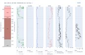
Due to the heterogeneity of the data in the property database there are frequently conflicting interpretations of net-to-gross, porosity and permeability for the same aquifer. This makes for a complex problem; to use all the data available introduces significant uncertainty and artefacts in the maps but to start selecting which data to use requires a system to identify potential erroneous data, inspect the data and track which data points we have inspected and decided to remove.
Through a combination of automatic anomaly detection, manual inspection and the development of specific software to facilitate this process an effective and traceable QC process was developed. For the current release v3.1 the QC was successfully applied to eight aquifers, which represent the most promising aquifers for geothermal in the Netherlands:
- Nieuwerkerk Formation, Alblasserdam Member (SLDNA)
- Nieuwerkerk Formation, Delft Sandstone Member (SLDND)
- Main Buntsandstein, Hardegsen Formation (RBMH)
- Main Buntsandstein, Upper Detfurth Sandstone Member (RBMDU)
- Main Buntsandstein, Lower Detfurth Sandstone Member (RBMDL)
- Main Buntsandstein, Upper Volpriehausen Sandstone Member (RBMVU)
- Rotliegend (Upper) Slochteren Formation (ROSL, ROSLU)
- Rotliegend Lower Slochteren Formation (ROSLL)
Work is continuing to complete this data QC process for all the aquifers of interest within ThermoGIS. This will be a part of a future ThermoGIS release.
SCAN Data
The SCAN programme by EBN is an effort to reduce uncertainties in the subsurface of the Netherlands through collecting seismic data and drilling boreholes in previously poorly surveyed areas. This makes the SCAN data particularly valuable as there is a large suite of modern measurements made in regions which are relatively data poor.
In ThermoGIS version 3.1 data from the SCAN wells were utilized for the first time:
| Well | Stratigraphy | NTG [-] |
Porosity [%] |
Permeability [mD] |
|---|---|---|---|---|
| AMS-01 | ROSL_ROSLU | 0.91 | 18.3 | 152 |
| ASD-01 | ROSL_ROSLU | 1.00 | 15.9 | 42 |
| BLT-01 | ROSL_ROSLU | 1.00 | 16.0 | 45.6 |
| EDE-01 | ROSL_ROSLU | 1.00 | 26.5 | 1546 |
| ORO-01 | NLDOBR | 0.88 | 36.1 | 141 |
| ORO-01 | NMRUBE | 0.96 | 33.2 | - |
| SVG-01 | NLLAOR | 0.34 | 18.6 | - |
This represents a fraction of the property information available due to the new SCAN wells. Data from the Milheeze (MHZ-01) and Heesch (HEE-01) wells, and data from other reservoirs that were targeted in the listed wells, will be used in the next ThermoGIS release
Interpolation method
To make property maps (which are planes) from the property data (which are points) an interpolation method is required; ThermoGIS has previously utilised Kriging along with empirical relationships between porosity and maximum burial depth, and between porosity and permeability. This methodology has significantly changed; Kriging is still utilised, but now it is universal Kriging with drift. Instead of prescribing an empirical relationship between porosity-max burial and porosity-permeability an integrated workflow is used to convert from max-burial to porosity and from porosity to permeability while Kriging the residuals between these drift fields. The method uses the package gstools which was extended and integrated in a python workflow.
Example of the application of the interpolation
Take the following synthetic example on the figure below. The green line f(x) is the 'True' function that we are trying to estimate.
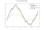
In this synthetic example the function is known but, of course, in reality it is unknown:
𝑓(𝓍) = 3 sin(2𝓍π) + 2𝓍
The red points are the observed data, which have noise added to them. This noise represents random uncertainty due to imperfect measurements. Uniform random noise between -0.5 and +0.5 has been added to the True function.
The filled orange line μ(x) is the drift function, which is provided by the subsurface specialist (or fitted to data if no other option is available). The specialist believes that this function is correlated to the 'truth' function. In this example the function is:
μ(𝓍) = sin(2𝓍π) + 𝓍
(Note how μ(x) has the same form, but different coefficients to f(x))
The Universal Kriging algorithm will first fit coefficients to μ(x) to estimate the drift field (orange dotted line in figure 2):
μ'(𝓍) = α + βμ(𝓍)
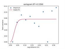
Then the residual between the observed data and the drift field is calculated. A variogram is fitted automatically (Figure 3) and the residual is Kriged and added back to the drift field, providing a local improvement on the drift.
After this process we get an estimate of the 'True' function and an uncertainty on this estimate, which is shown by the blue line on Figure 2. It can be seen that this blue line follows the truth fairly well, but it is fitting the observations too closely. This is because the observational error was set too low – an example of having too much confidence in the quality of the data. In this initial example, the observational error has been set to 0.1 while the true observational error is much larger: 1.0 in reality. The final estimate is overfitting the data.
If the observational error is set to 1.0, the following result is obtained (Figure 4):
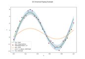
The result is an estimate that:
- Follows an expert provided drift function;
- Fits observed data to within (provided) observational error;
- Through Kriging can provide an uncertainty band in the final estimate;
- Utilises automatic variogram fitting to remove subjective model choices and simplify the workflow.
Automatic Variogram Estimation
Multiple variogram models (Gaussian, Exponential, Spherical, Matern, Stable) are tested and the one which fits the data best is selected. Now with this automated variogram selection algorithm variogram selection is dependent entirely on the data.
Gstools provides the algorithms to estimate the bin values and to fit variogram models accordingly. In the ThermoGIS workflow this functionality is simply extended to try multiple types of models and select the one which performs the best.
Effect of observational uncertainty
With the new framework it is possible to add uncertainty to individual data points. This means meta-information on each observed value can be used to produce an estimate of the uncertainty on that observation which can then be included in the Kriging algorithm. The improvement in the final estimate can be seen when comparing figure 2 to figure 4.
Aquifers with too few data
In previous ThermoGIS maps, Kriging was utilised irrespective of the amount of data points available for an aquifer. This is not statistically valid. Therefore, for aquifers and properties with less than (an arbitrary) 10 property observations a mean and standard deviation of the data is taken and a 'flat' map (i.e., with a constant value) is produced.
For aquifer-properties with less than 5 property observations the mean and standard deviation of the Group data is taken.
Table 2 shows the amount of well data per property, per aquifer and which methodology was utilised for the current ThermoGIS version.
| Aquifer | NWells NtG | NtG method | NWells Porosity | Poro method | NWells Perm | Perm method |
|---|---|---|---|---|---|---|
| DCD | 25 | Krige | 60 | Krige | 8 | Mean and SD Aquifer |
| DCH | 6 | Mean and SD Aquifer | 29 | Krige | 20 | Krige |
| SLDNA | 40 | Krige | 52 | Krige | 38 | Krige |
| SLDND | 36 | Krige | 36 | Krige | 32 | Krige |
| KNNSL | 9 | Mean and SD Aquifer | 73 | Krige | 19 | Krige |
| KNGLG_KNGLS | 7 | Mean and SD Aquifer | 42 | Krige | 11 | Krige |
| KNNSB | 25 | Krige | 33 | Krige |
14 |
Krige |
| KNNSF | 32 | Krige | 117 | Krige | 25 | Krige |
| KNNSG | 4 | Mean and SD Group | 64 | Krige | 7 | Mean and SD Aquifer |
| KNNSP | 10 | Mean and SD Aquifer | 202 | Krige | 16 | Krige |
| KNNSR | 36 | Krige | 69 | Krige | 44 | Krige |
| KNNSY | 12 | Krige | 70 | Krige | 11 | Krige |
| RBSHN | 1 | Mean and SD Group | 1 | Mean and SD Group | 1 | Mean and SD Group |
| RBMDL | 50 | Krige | 105 | Krige | 24 | Krige |
| RBMDU | 19 | Krige | 25 | Krige | 5 | Mean and SD Group |
| RBMH | 47 | Krige | 56 | Krige | 24 | Krige |
| RBMVL | 68 | Krige | 191 | Krige | 27 | Krige |
| RBMVU | 41 | Krige | 51 | Krige | 15 | Krige |
| RNROF | 52 | Krige | 64 | Krige | 49 | Krige |
| RNSOB | 59 | Krige | 36 | Krige | 22 | Krige |
|
ROSL_ROSLU |
267 | Krige | 543 | Krige | 220 | Krige |
| ROSLL | 50 | Krige | 77 | Krige | 19 | Krige |
| NLDOBR | 15 | Krige | 17 | Krige | 16 | Krige |
| NLDOOO | 1 | Mean and SD group | 3 | Mean and SD group | 0 | Mean and SD group |
| NLLAOR | 1 | Mean and SD group | 1 | Mean and SD group | 0 | Mean and SD group |
| NLLARE | 0 | Mean and SD group | 0 | Mean and SD group | 0 | Mean and SD group |
| NMVESO | 0 | Mean and SD group | 1 | Mean and SD group | 0 | Mean and SD group |
| NMVEVO | 0 | Mean and SD group | 7 | Mean and SD group | 5 | Mean and SD group |
| NMRUST | 0 | Mean and SD group | 0 | Mean and SD group | 0 | Mean and SD group |
| NMRUBE | 1 | Mean and SD group | 4 | Mean and SD group | 3 | Mean and SD group |
| NUBD | 18 | Krige | 15 | Krige | 15 | Krige |
| NUBG | 18 | Krige | 17 | Krige |
17 |
Krige |
Results
The resulting changes in the property maps are significant with respect to previous ThermoGIS versions. The combination of improved data quantity, quality and an improved interpolation method has meant that property maps have become more reliable. At the same time, the approach to producing maps has changed. For some aquifers and properties it must be concluded that knowledge of the spatial distribution of the properties is less well determined than previously thought. This means that for some aquifer-properties the resulting maps now display less spatial detail than before. Still, this better reflects our understanding of the subsurface, and therefore these new property maps are considered to be better representations of the subsurface.